PhD course
High throughput sequencing of non-model organisms
Course material for bioinformatics data analysis
04 Jun 2015
Alexander Jueterbock
Martin Jakt
Mapping and variant calling
Materials
Download PDF
Once you have assembled a draft genome, you can map your reads against it and identify potential read variants, like SNPs (Single Nucleotide Polymorphisms) and InDels (Insertions and Deletions). The library that you sequenced in this course is likely to represent a single diploid individual. Read variants, thus, occur at loci that differed between the mother and the father of this individual. Read variants become interesting when they are associated with certain environmental factors or phenotypes. This, however, requires sequencing several individuals of differing phenotypes or obtained from several environments.
Mapping with Bowtie2
To map reads against the assembled draft genome, we will use Bowtie2. Bowtie2 defaults to finding global alignments (no soft-clipping of terminal bases) and it allows for gaps in the alignment, thereby increasing mapping accurracy (Schlotterer et al. (2014) Nature Reviews Genetics). Although the aligner TMAP was specifically compiled for Ion Torrent data, in this tutorial we want use an aligner that can also be used with Illumina or SoliD data - as you are likely to work with sequencing data that were obtained from these platforms in the future. An alternative aligner that is currently widely used is BWA.
What you need for mapping are two fasta files, one containing the
quality-trimmed reads and the other containing the draft genome.
Create a new folder named Mapping (with mkdir) and copy the two
fasta files into it (with cp). For example:
mkdir Mapping

cp GenomeAssembly/IonTorrentDeNovoAssembly_d_results/\
IonTorrentDeNovoAssembly_out.unpadded.fasta \
Mapping/

cp RAWREADS_trimmed_trimmed.fq \
Mapping/

cd Mapping
In the Mapping folder, we first create an index for the reference genome using the following command:
bowtie2-build -f IonTorrentDeNovoAssembly_out.unpadded.fasta GENOMENAME
You can change GENOMENAME to whatever you like.
Now, to align the trimmed reads against the genome, use the following command:
nohup bowtie2 -p 1 \
-q \
--phred33 \
--sensitive \
--no-unal \
--al-gz FILE_Aligned.fq.gz \
--un-gz FILE_Unaligned.fq.gz \
--met-file MetricsFile.txt \
-x GENOMENAME \
-U RAWREADS_trimmed_trimmed.fq \
-S MAPPEDREADS.sam >Logfile.log &
Here an overview of the meaning of the used options:
-p 1- Causes Bowtie 2 to use a single thread. Depending on the number of users and libraries we will probably increase this.
-q- Informs the program that the reads to map are saved in fastq files.
--phred33- Sets the quality encoding of the fastq files to “Phred+33”.
--sensitive- sets several options at once regarding the seeding and other adjustments.
--no-unal- Suppress SAM records for reads that do not align.
--al-gz- Write unpaired reads that align at least once to to the specified file.
--un-gz- Write unpaired reads that failed to align to the specified file.
--met-file- Write bowtie2 metrics to Metricsfile.txt.
-x- Specifies the name of the genome.
-U- Specify the unpaired reads to align (can contain a comma-separated list of several fq files).
-S- Specify the sam file to which the alignment shall be saved.
You can’t set the exact number of mismatches in the seed, but you can adjust the mismatch penalty.
The program should run no longer than 10-20 mins. The resulting output file will be in the SAM format. For a detailed description of this format, see here.
Filter mappings
To remove unmapped reads, reads below a mapping quality of 20, and reads that were not aligned uniquely (reads that were mapped to >1 places in the genome), use the python script Bowtie2Filtering.py:
Bowtie2Filtering.py -mq -u -a -s MAPPEDREADS.sam
Your filtered reads will be saved in MAPPEDREADSfiltered.sam
Alternatively, you can use samtools to filter out reads with a mapping quality <20:
samtools view -Sh -q 20 -o MAPPEDREADS_QualityAbove20.sam MAPPEDREADS.sam
Options:
-S- Input is in the sam format
-h- Include the samfile header in the output
-q- Skip alignments with a mapping quality below 20
Removing duplicate reads
After quality-trimming, we counted the fraction of duplicate reads. Duplicate reads have the same start and end coordinates and map to the same region. Duplicates result from primer or PCR bias towards these reads. As they can skew genotype estimates, they should be removed before SNP calling.
To remove duplicates, we will use ‘MarkDuplicates’ from the Picard command line tools. An alternative tool is samtools rmdup, which considers single-end reads to be duplicates when their mapping locations are the same - even if the base composition differs between the reads.
First, we need to convert our sam file to a bam file (a binary, compressed version of a sam file that is not human-readable) and sort the reads by the leftmost mapping coordinates.
samtools view -bSh MAPPEDREADS.sam  > MAPPEDREADS.bam
samtools sort MAPPEDREADS.bam MAPPEDREADS_sorted
Meaning of the options:
-b- output in bam format
-S- input in sam format
-h- include the header in the output
Then, you can use the java script ‘MarkDuplicates.jar’ from Picard tools to remove the duplicates from the sorted bam file:
picard-tools MarkDuplicates \
INPUT=MAPPEDREADS_sorted.bam \
OUTPUT=MAPPEDREADS_dedup.bam \
METRICS_FILE=MAPPED_metricsfile \
ASSUME_SORTED=true \
VALIDATION_STRINGENCY=SILENT \
REMOVE_DUPLICATES=true
Duplication metrics will be written to the MAPPED_metricsfile.
Re-alignment around indels
Reads that are spanning InDels are often misaligned and can result in false SNPs (see Schlotterer et al. (2014) Nature Reviews Genetics). These reads should be removed or re-aligned. We have not enough time to re-align the reads in this course but the required steps (using GATK) are described in detail here: http://sfg.stanforde.edu/SFG.pdf.
Visualizing alignments
Samtools tview: command-line viewer
The command line tool samtools tview allows you to view your
alignments directly in the command line window. What you need is the
reference genome (fasta file) and the sorted and deduplicated
alignment file (bam file). First, you need to index the bam file
before using samtools tview:
samtools index MAPPEDREADS_dedup.bam

samtools tview MAPPEDREADS_dedup.bam \
IonTorrentDeNovoAssembly_out.unpadded.fasta
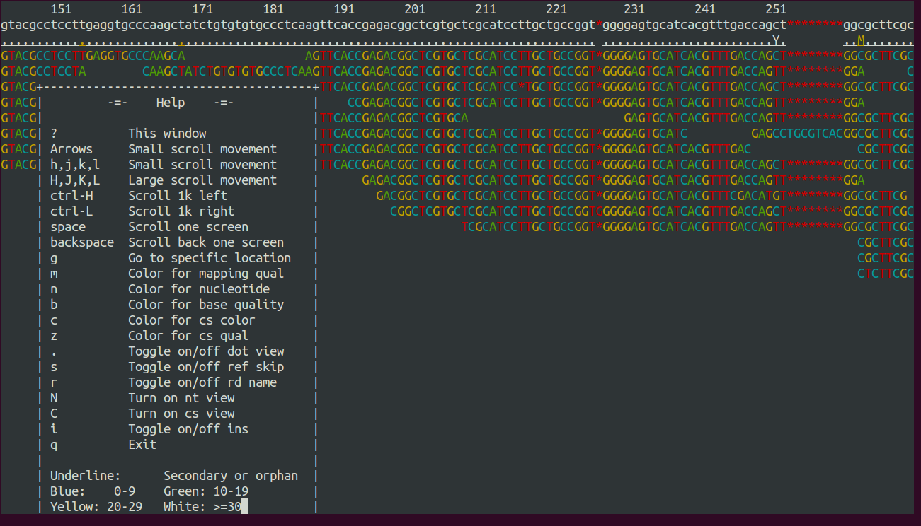
Fig. 1 shows a screenshot of tview. When you hit the ? on
your keyboard, you will see the range of options to navigate through
the alingment. You can change the contig that you are looking at by
hitting g and then enter in the Goto-window the name of the contig,
like ‘IonTorrentDeNovoAssembly_c3’. You can exit the alignment viewer
by hitting q.

Figure 1: Screenshot of tview
IGV: viewer with a graphical user interface
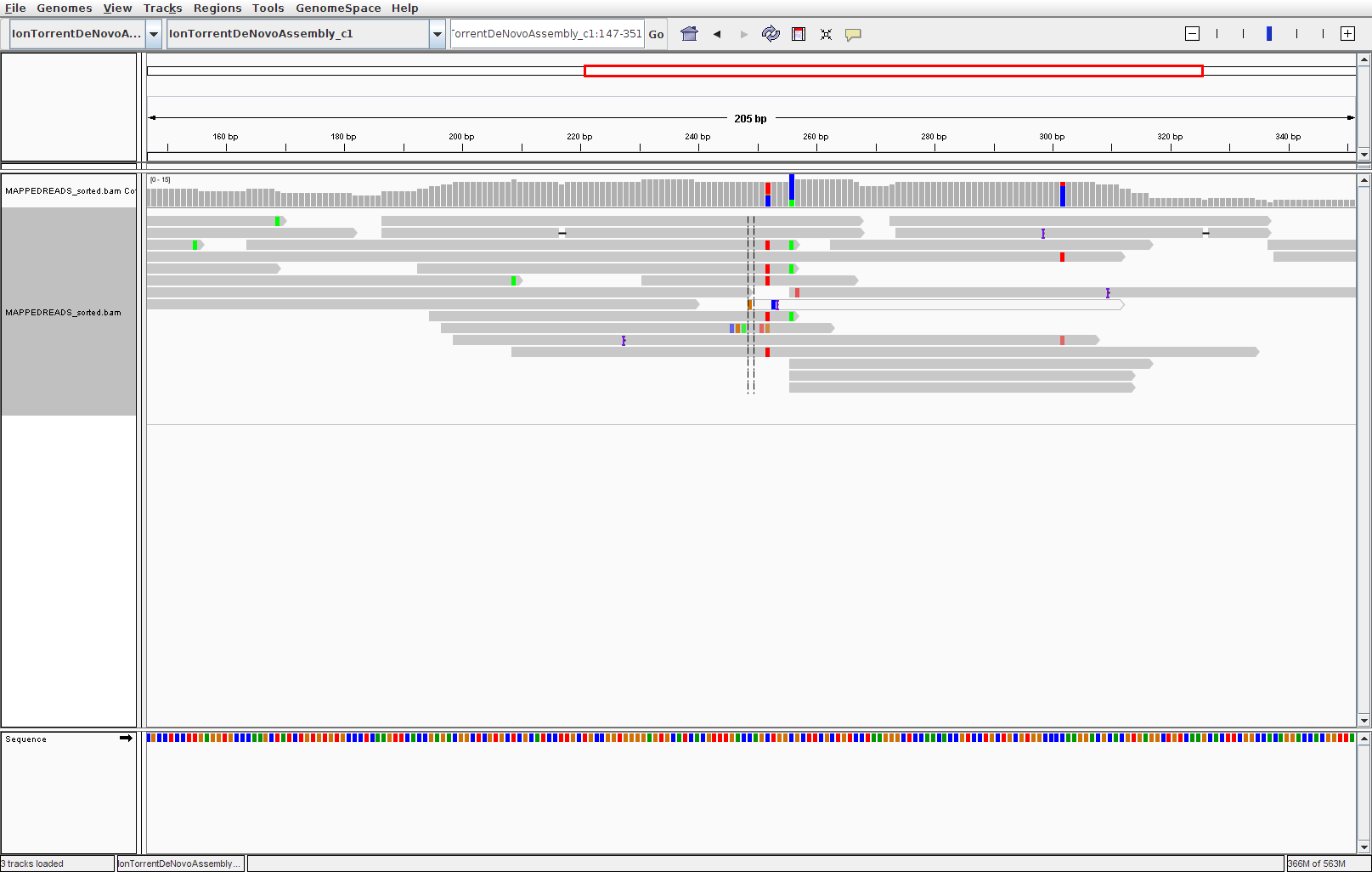
I bet that many of you prefer to look at the alignment in a graphical user interface. A decent free alignment viewer is igv, the Integrative Genomics Viewer (see Fig. 2 for a screenshot). Once you have registered, you can launch the program with Java Web Start. We can’t promise that this works well in the course, since everything that relies on a graphical user interface can be quite slow when using a remote connection. Thus, you might want to download the required files (deduplicated SAM file and reference genome) and try out igv on your private computer. The interface is pretty much self-explanatory. To look at the alignment, you first need to load a genome and then add the mapped, sorted and indexed bam file.

Figure 2: Screenshot of igv with reads aligned to a reference and colored mismatches
BONUS: SNP calling with samtools mpileup and bcftools
A widely used tool to identify sequence variants is samtools
mpileup. See here for an overview of its options. The tool samtools
mpileup defaults to creating a pileup file, which summarizes aligned
base calls in text format (see here for a detailed characterization of
a pileup file http://samtools.sourceforge.net/pileup.shtml). If you
call samtools mpileup with the -u or -g option, instead, the
output format is a vcf or bcf (compressed binary version of vcf) file;
vcf stands for ‘variant call format’. Its format specifications are
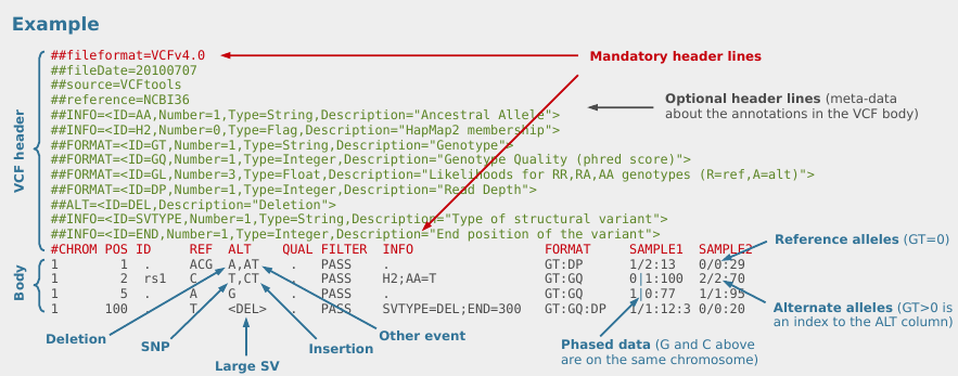
described here and summarized in Fig. 3.
The first step for calling SNPs from your aligned and deduplicated reads is:
samtools mpileup -g \ -f \ IonTorrentDeNovoAssembly_out\ .unpadded.fasta \ -q 20 \ -Q 20 \ -t DP \ -t SP \ MAPPEDREADS_dedup.bam > MAPPEDREADS_dedup.bcf
The chosen options are described on this page. By setting the -t SP and
-t DP tags, samtools mpileup provides:
-t SP- per-sample Phred-scaled strand bias P-value
-t DP- per sample read depth
To call SNPs from the bcf file, we use bcftools:
bcftools call -vm -V indels MAPPEDREADS_dedup.bcf > MAPPEDREADS_variants.vcf
Options:
-v- Output variant sites only
-V indels- Skip indels
-m- model for multiallelic and rare-variant calling

Figure 3: VCF file overview from Petr Danecek
To count how many SNPs were found, use the following command:
grep -v -c '^#' MAPPEDREADS_variants.vcf
The option -v in combination with ^# excludes all header lines
that start with (^) the #-sign. With the -c option, grep counts
the lines instead of writing them out.
To filter out SNPs that are low quality or covered by low depth, we
can use the vcfutils.pl varFilter that comes with samtools:
vcfutils.pl varFilter -d 5 -w 3 -Q 20 MAPPEDREADS_variants.vcf > MAPPEDREADS_variants_filtered.vcf
Options used:
-d 5- minimum read depth of 5
-w 3- SNP within 3 bp around a gap to be filtered. This may be an alternative solution to re-alignment around indels
-Q 20- minimum mapping quality of 20
Another useful option can be:
-1 0.0001- min P-value for strand bias (given the PV4-tag in the
vcf file). We obtained the PV4-tag by setting the
-t SPtag insamtools mpileup. This option filters out the SNPs that have a strong strand-bias: SNPs that are supported by one strand and not the other.
Count how many SNPs are left after filtering
grep -v -c '^#' MAPPEDREADS_variants_filtered.vcf
The SNPs can be visualized with IGV. For this, we first need to compress and index the vcf files:
bgzip -c \
MAPPEDREADS_variants_filtered.vcf \
> MAPPEDREADS_variants_filtered.vcf.gz

tabix \
-p vcf \
MAPPEDREADS_variants_filtered.vcf.gz
Open IGV and load the indexed bam file and the indexed vcf file.