If you want to identify sequence variants like SNPs (Single Nucleotide Polymorphisms) or InDels (Insertions and Deletions) in your sequencing data, you want to avoid regions of too low coverage. The lower the coverage the more difficult it becomes to discriminate sequencing errors from real sequence variants.

Too high coverage, however, may also be problematic and this blog post introduces a python script that can help to identify the problematic high coverage in pileup files. Pileup format is a text-based format that summarizes base calls of aligned reads to a reference sequence (see here for a detailed description: http://samtools.sourceforge.net/pileup.shtml)

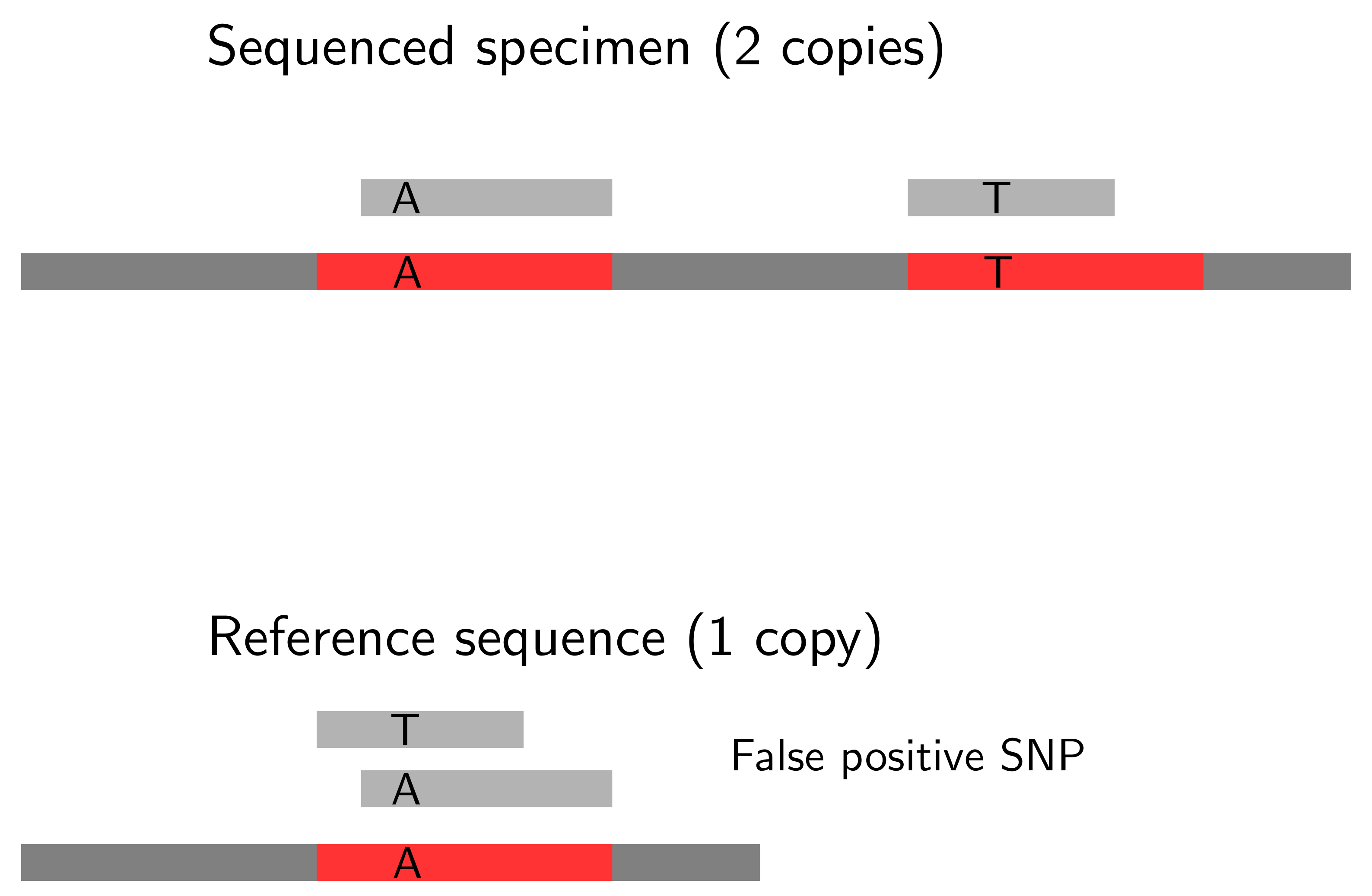
Extraordinarily high coverage can result from copy number variations that will lead to false positive variant calls. This gets more clear in Figure Fig.CNV. Here, the two gene copies in the sequenced individual will map to the single gene copy in the reference sequence. This region will be covered by a much higher number of reads than other regions of the reference sequence, and will be identified as a SNP.

::: {.center} {width=”500px” title=”CNV” alt=”CNV” align=”middle”} :::

There are different approaches to avoid calling false SNPs due to copy number variation. The NGS analysis pipeline popoolation for pooled populations, for example, allows to subsample a pileup file to a uniform coverage with the script subsample-pileup.pl. Others have set an upper coverage threshold, like twice the mean coverage (Lynch et al., 2014), the upper 2% of all coverages (Tobler et al. , 2014) or the mean coverage plus two standard deviations (Beissinger et al. , 2014). Sites with a coverage above this threshold were discarded before calling variants. The python script thresholds.

References:

• Lynch, Michael, et al. “Population-genetic inference from pooled-sequencing data.” Genome biology and evolution 6.5 (2014): 1210-1218. (Link)

• Tobler, Ray, et al. “Massive habitat-specific genomic response in D. melanogaster populations during experimental evolution in hot and cold environments.” Molecular biology and evolution 31.2 (2014): 364-375. (Link)

• Beissinger, Timothy M., et al. “A genome-wide scan for evidence of selection in a maize population under long-term artificial selection for ear number.” Genetics 196.3 (2014): 829-840. (Link)

Download

You can download the script PileupCoverageOverview.py from https://gist.github.com/alj1983/2f0ce22fa28aef4a0922/download

How to use it?

usage: PileupCoverageOverview.py [-h] [-p PILEUP] [-ma MAX] [-mi MIN]

Creates a cumulative histogram on read coverage (excluding coverage of 0)

optional arguments: -h, –help show this help message and exit -p PILEUP, –pileup PILEUP pileup file name -ma MAX, –max MAX maximum coverage to be shown -mi MIN, –min MIN minimum coverage to be shown

The -ma and -min options specify the upper and lower coverage thresholds that will be shown in a cumulative histogram. Independent of these options, however, PileupCoverageOverview.py will always return the following coverage measures (numbers give an example):

Coverage - mean: 220.00 Coverage - max: 12312 Coverage - min: 1 Coverage - mean-2stddev: -760 Coverage - mean+2stddev: 1200 Coverage - upper 2%: 2020 Coverage - lower 2%: 1

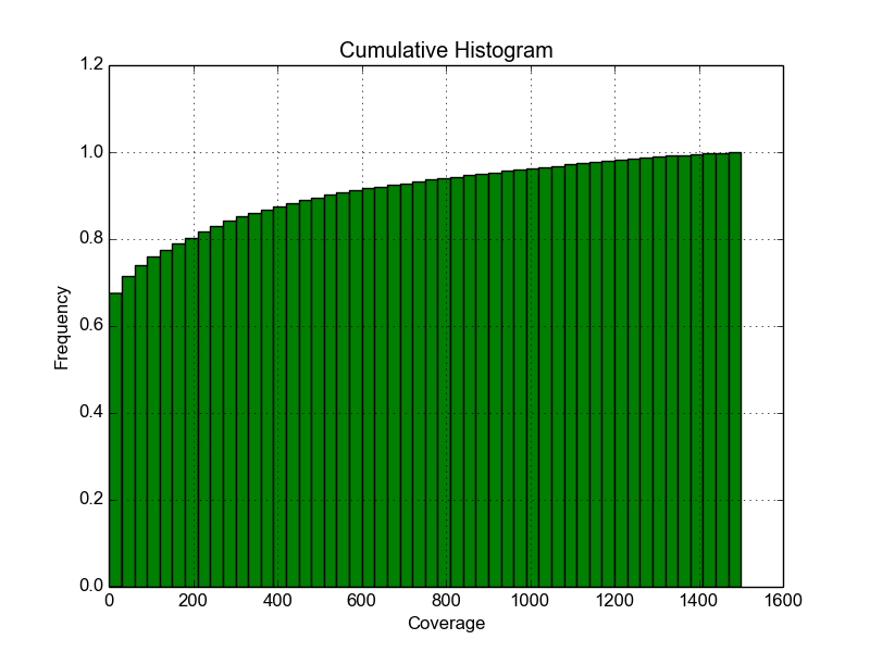
Fig. Fig.Histogram shows the cumulative histogram of read coverages, that is based on the same input file. Here for example, 90% of all reads had a read-coverage below 600.

::: {.center} {width=”500px” title=”histogram” alt=”histogram” align=”middle”} :::

Code

import re # to use regular expressions import math import argparse # To allow users setting flags in order to define what to filter for. from pylab import figure, title, xlabel, ylabel, hist, axis, grid, savefig # to draw a historgram

parser = argparse.ArgumentParser(description=”Creates a cumulative histogram on read coverage (excluding coverage of 0) and prints out upper and lower coverage thresholds”) parser.add_argument(“-p”,”–pileup”, help=”pileup file name”) parser.add_argument(“-ma”,”–max”, help=”maximum coverage to be shown”) parser.add_argument(“-mi”,”–min”, help=”minimum coverage to be shown”) args=parser.parse_args()

Define the search patterns:

PileupFileNamePattern = re.compile(‘(.*).pileup’)

def Coverages(pileupfile,maximum,minimum): ‘’’ Creates a cumulative histogram on read coverage (excluding coverage of 0) and prints out upper and lower coverage thresholds ‘’’ pileup=open(pileupfile) OutfilePrefix1 =PileupFileNamePattern.match(pileupfile) # define outfile OutfilePrefix=OutfilePrefix1.group(1)
Coverage=[] #Create an empty list for line in pileup: line=line.strip() splitted=line.split(‘\t’) # Split the lines by tab separators if abs(int(splitted[3])) > 0: # excluding all coverages of 0 Coverage.append(abs(int(splitted[3]))) # Pick out the 4th column, which is the number of reads that covered this position # Remove coverages of 0 CoverageAboveZero=[] for c in Coverage: if c>0:
CoverageAboveZero.append(c) # sort the coverages CoverageAboveZeroSorted = CoverageAboveZero.sort() TotalBasesCovered = len(CoverageAboveZeroSorted) # Identify the lower 2% limit LowerLimit=CoverageAboveZeroSorted[int((0.02TotalBasesCovered)-1)] # Identify the upper 2% limit UpperLimit=CoverageAboveZeroSorted[int((0.98TotalBasesCovered)-1)] # Calculating the standard deviation mean=float(sum(CoverageAboveZeroSorted)/len(CoverageAboveZeroSorted)) total = 0.0 for value in CoverageAboveZeroSorted: total += (value - mean) ** 2 stddev = math.sqrt(total / (len(CoverageAboveZeroSorted)-1)) print pileupfile, ‘Coverage - mean:’, ‘%10.2f’ % mean print pileupfile, ‘Coverage - max:’, ‘%10i’ % max(CoverageAboveZeroSorted) print pileupfile, ‘Coverage - min:’, ‘%10i’ % min(CoverageAboveZeroSorted) print pileupfile, ‘Coverage - mean-2stddev:’, ‘%10i’ % mean-2stddev print pileupfile, ‘Coverage - mean+2stddev:’, ‘%10i’ % mean+2stddev print pileupfile, ‘Coverage - upper 2%:’, ‘%10i’ % UpperLimit print pileupfile, ‘Coverage - lower 2%:’, ‘%10i’ % LowerLimit

 # Drawing the historgram
 figure()
 hist(CoverageAboveZeroSorted, range=(minimum,maximum), bins=50, histtype='bar', facecolor='green', normed=1,cumulative=1)
 title('Cumulative Histogram')
 xlabel('Coverage')
 ylabel('Frequency')
 axis()
 grid(True)
 savefig(OutfilePrefix + 'Coverage_Histogram.png')

Coverages(str(args.pileup),int(args.max),int(args.min))